Research 5 - illustrate the concept of conditional, joint, marginal relative frequency

To illustrate the concepts of conditional, marginal and relative frequency we must start from a bivariate distribution. A bivariate distribution reports in a contingency table the frequencies of all the possible values assumed by two attributes of a certain statistical set. A generic bivariate distribution is the following:

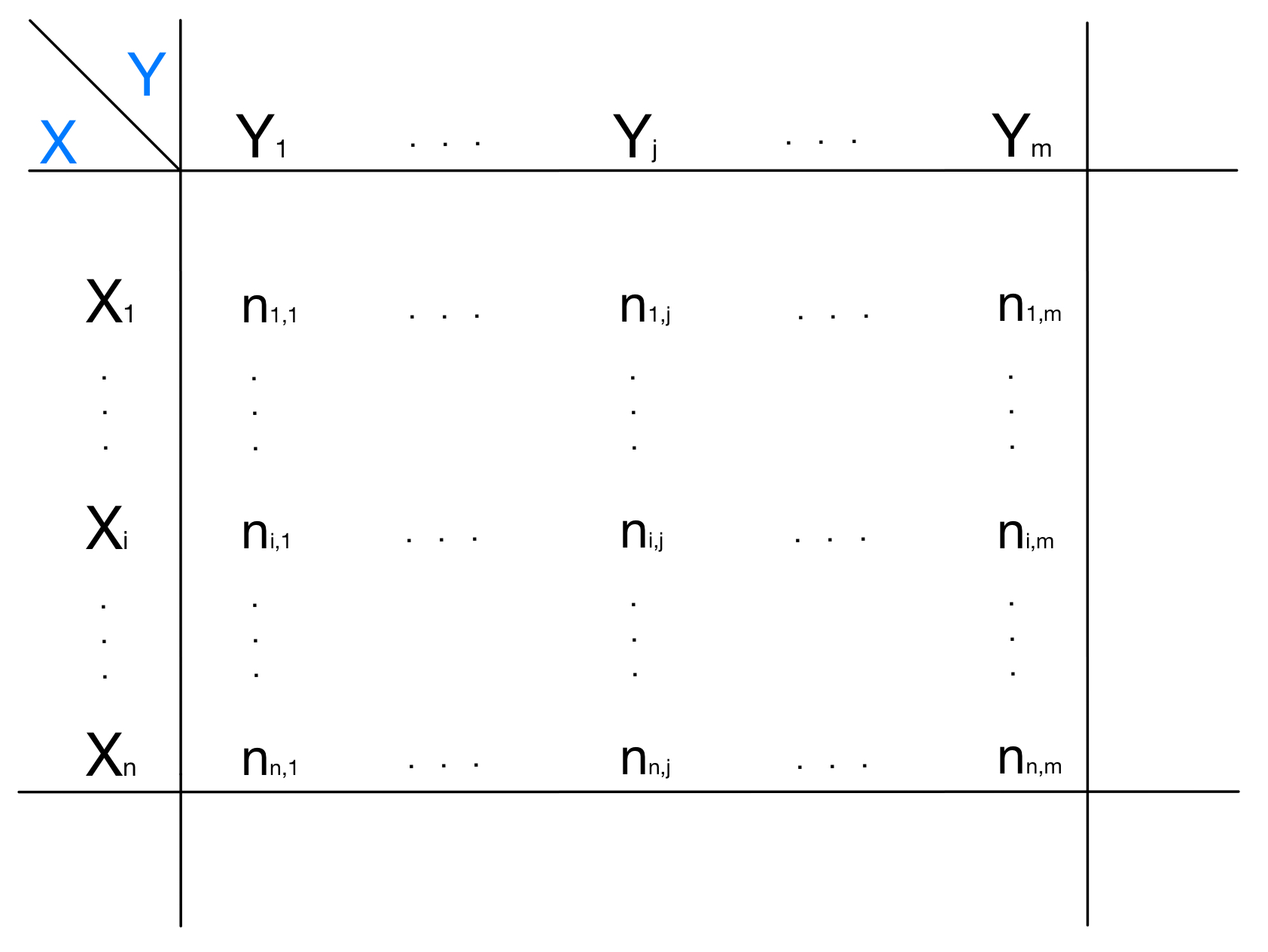
In this generic representation, we have the two attributes $X$ and $Y$. In the cell $(i,j)$ of the table it is reported the frequency of those statistical units that have $X_i$ as a value for attribute $X$ and $Y_j$ as a value for attribute $Y$. In this generic example the reported frequencies are absolute frequencies, meaning that they represent the exact number of statistical units having those values for those attributes. Much more interesting is to study the relative frequencies, that are the above absolute frequencies divided for the total number of the statistical units considered.

In order to explain better the concept of conditional, joint and marginal frequencies let’s take, as an example, the following bivariate distribution:

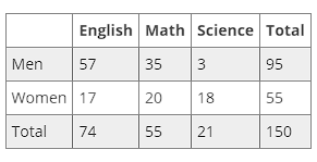
The distribution was created on a total set of 150 people. The attributes considered are their sex and the subject they considered the most difficult at school. The frequencies reported are absolute frequencies.

The joint relative frequency of two values is the absolute frequency of those two values, divided for the total number of units considered to create the table. For example if we consider the value “Men” for the attribute “Sex” and the value “Math” for the attribute “Subject”, the joint relative frequency of “Men” and “Math” will be:

\[freq(Men \cap Math) = \dfrac{35}{150} = 0,23\]

This intuitively means that 23% of the units have at the same time the value “Men” for the attribute “Sex”, and the value “Math” for the attribute “Subject”

Once we have seen this example, it’s now easy to generalize and say that, given two attributes $X$ and $Y$, the joint relative frequency of two generic values $X_i$ and $Y_j$ can be calculated as:

\[f_{i,j} = freq(X_i \cap Y_j) = \dfrac{n_{i,j}}{N}\]

Where n_{i,j} is the number of units that have $X_i$ as the value for $X$ and $Y_j$ as the value for $Y$, and $N$ is the total number of statistical units considered.

The marginal relative frequency, instead, refers just to one attribute, ignoring the other: it represents the frequency of a certain value for one of the two attributes, ignoring the value assumed by the other attribute. In order to calculate it, we need to sum all the absolute frequencies in a certain row (if the attribute considered is the “row attribute”) or in a certain coulmn (if the attribute considered is the “column attribute”), to divide then by the total number of units.

Referring to the distribution in the picture, the marginal relative frequency for the value “Women” of attribute “Sex” can be calculated as:

\[freq(Women) = \dfrac{55}{150} = 0,37\]

Notice how we made the sum of all the absolute frequencies reported in the row relative to the value “Women”, to then divide by the total number of units. We obtained this way the relative frequency of the value “Women”: we can say that 37% of the units have the value “Women” for the attribute “Sex”, independently from the value assumed by the attribute “Subject”. If we generalize to the generic attributes $X$ and $Y$:

\[f_{i,.} = freq(X_i) = \dfrac{1}{N}(\sum_{j = 1}^{m}n_{i,j}) = \dfrac{N_{i,.}}{N}\] \[f_{.,j} = freq(Y_j) = \dfrac{1}{N}(\sum_{i = 1}^{n}n_{i,j}) = \dfrac{N_{.,j}}{N}\]

In the above notation, the dot (“.”) represents the attribute on which we operate the marginalization and that we do not consider in the calculation of the frequency.

Finally, the conditional relative frequency is the frequency of a certain value of one of the two attributes, but this time calculated over a subset of the statistical units. This subset is created by considering only those units that have a specific value for the other attribute. Referring to the above distribution, the frequency of the value “Men” for attribute “Sex”, conditioned on the value “English” for the attribute “Subject”, is the following:

\[freq(Men|English) = \dfrac{57}{74} = 0,77\]

We can notice how the numerator is the joint frequency of “Men” and “English”, because we have to consider only those men who have “English” as the value for attribute “Subject”, while the denominator is the absolute marginal frequency of the value “English”, since we want the cardinality of the subset composed by those units that have “English” as the value of the attribute “Subject”.

If we again generalize to the generic attributes $X$ and $Y$:

\[f_{i/j} = freq(X_i|Y_j) = \dfrac{n_{i,j}}{N_{.,j}}\] \[f_{j/i} = freq(Y_j|X_i) = \dfrac{n_{i,j}}{N_{i,.}}\]

Where $N_{i,.}$ and $N_{.,j}$ are respectively the cardinality of the subset of the units having the value $X_i$ for the attribute $X$ and the cardinality of the subset having the value $Y_j$ for the attribute $Y$.

It’s now easy to verify that:

\[f_{i/j} = \dfrac{f_{i,j}}{f_{.,j}} = \dfrac{freq(X_i \cap Y_j)}{freq(Y_j)}\] \[f_{j/i} = \dfrac{f_{i,j}}{f_{i,.}} = \dfrac{freq(X_i \cap Y_j)}{freq(X_i)}\]

In fact:

\[f_{i/j} = \dfrac{freq(X_i \cap Y_j)}{freq(Y_j)} = \dfrac{\dfrac{n_{i,j}}{N}}{\dfrac{N_{.,j}}{N}} = \dfrac{n_{i,j}}{N_{.,j}}\] \[f_{j/i} = \dfrac{freq(X_i \cap Y_j)}{freq(X_i)} = \dfrac{\dfrac{n_{i,j}}{N}}{\dfrac{N_{i,.}}{N}} = \dfrac{n_{i,j}}{N_{i,.}}\]

References
[1] https://study.com/learn/lesson/conditional-joint-marginal-relative-frequency-overview-comparison-examples.html#:~:text=Marginal%20relative%20frequency%20is%20the%20ratio%20of%20the%20sum%20of,total%20or%20a%20column%20total.

Research 6 - illustrate the concept of statistical independence and the resulting mathematical relationship between the above frequencies

Let’s take a bivariate distribution. As we have seen in the research above, a bivariate distribution shows the distribution of a pair of attributes. Those attributes are independent if the value of one of them has no effect on the frequency of the values of the other one and vice versa.

Let’s take, as an example, the following distribution:

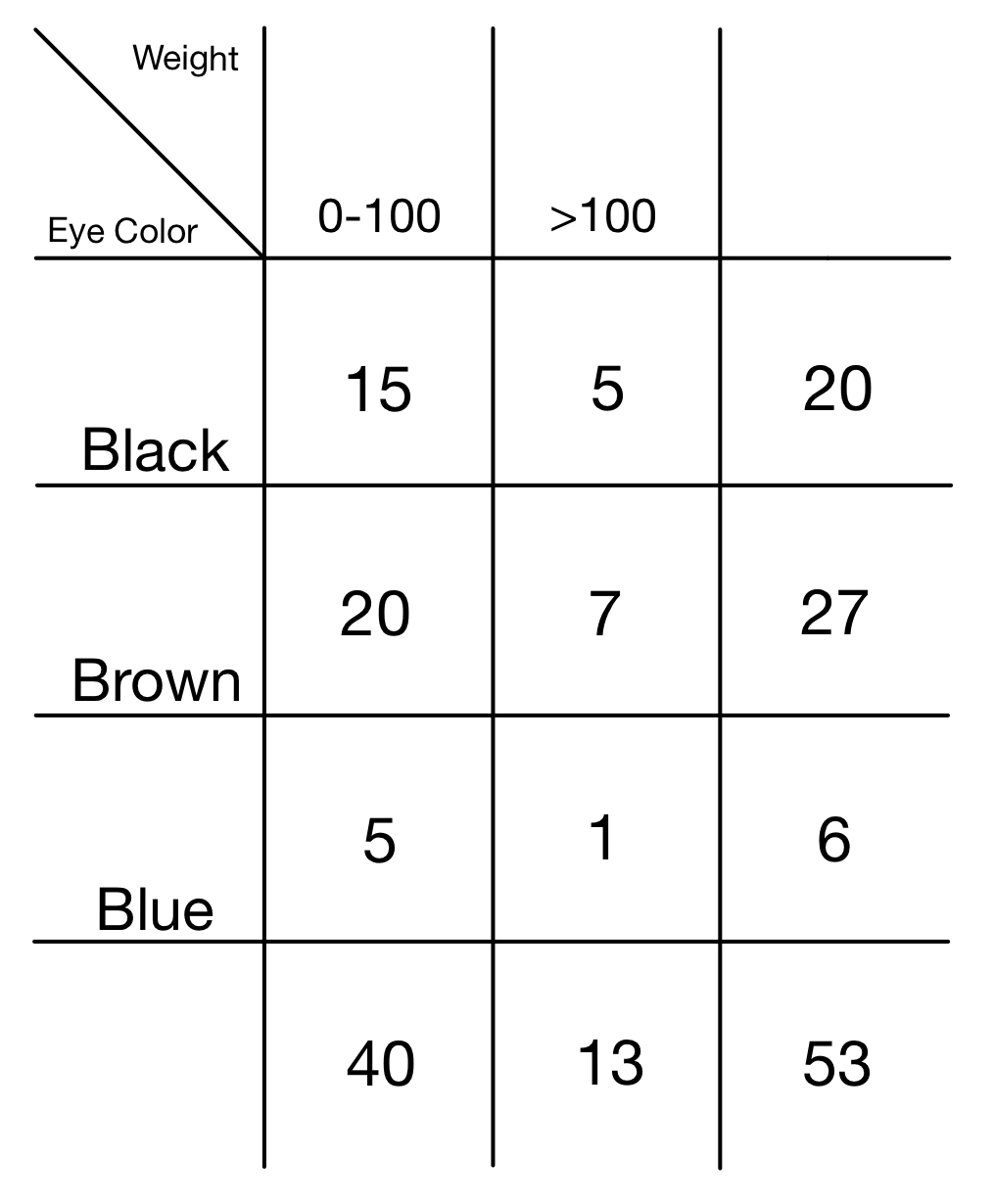
It’s easy to imagine how the two attributes “Eye color” and “Weight” are not correlated by any relation. This can be seen in the distribution: if we consider the single rows or the single columns, although the absolute values reported are of course different, they are proportioned. If we put in a graph, for example, the absolute conditional distributions of attribute “Weight” over the various values assumed by the attribute “Eye Colour”, the shape of those graphs will be the same: the conditional absolute distributions do not vary. This can be better seen if we compute conditional relative frequencies.

In fact, the concept of independence is strictly related to the concepts of joint, marginal and conditional relative frequency that we described above. We said that joint relative frequency of values $X_i$ and $Y_j$ is calculated as:

\[f_{i,j} = freq(X_i \cap Y_j) = \dfrac{n_{i,j}}{N}\]

But if the two attributes $X$ and $Y$ are independent, we will have that:

\[f_{i,j} = freq(X_i \cap Y_j) = freq(X_i)freq(X_j)\]

Where $freq(X_i)$ is the marginal relative frequency of $X_i$ and $freq(Y_j)$ is the marginal relative frequency of $Y_j$. If we compute the joint frequencies of values “Black” and “0-100” we can see this clearly:

\[f_{i,j} = freq(Black \cap 0-100) = \dfrac{15}{53} = 0,28\]

But also:

\[f_{i,j} = freq(Black)freq(0-100) = \dfrac{20}{53}\dfrac{40}{53} = 0,28\]

Another important mathematical consequence of independence is related to conditional relative frequencies, as we stated before. In fact, if $X$ and $Y$ are independent, we will have that:

\[f_{i/j} = freq(X_i|Y_j) = freq(X_i)\] \[f_{j/i} = freq(Y_j|X_i) = freq(Y_j)\]

In case of independence, the relative frequency of any value of an attribute, conditioned to any value of the other attribute, will be equal to the marginal relative frequency of the value considered. This can be easily seen in the table above, if we condition the frequency of value “Brown” on the value “0-100”

\[freq(Brown) = \dfrac{27}{53} = 0,5\] \[freq(Brown|0-100) = \dfrac{20}{40} = 0,5\]

This result allows us to say with more precision what we stated initially: even if row by row (or column by column) the absolute distributions may seem different, if we condition on the row value (or on the column value) we see that the resulting distribution is identical to the marginal distribution. This makes evident that the two attributes are independent: the results i obtain if i consider just a conditioned subset of my statistical units are the same i obtain with the whole set. This means that the conditioning attribute has no influence on the conditioned one.