Research 4 - Concept of distribution. Univariate and multivariate. Conditional and marginal distributions.

When talking about distribution in Statistics we may refer to two different concepts:

1. Probability distribution

2. Frequency distribution

The first is more related to Probability Theory, and consists in a function that gives the probabilities of occurrence of different possible outcomes in an experiment. The second, instead, is more related to actual Statistics, and is a representation showing all the possible values a certain attribute can assume and how often those values occur. In this research, we focus on frequency distribution.

Given a certain population, we can create a dataset that summarizes some informations about that population. A dataset (or data matrix) is composed by rows and columns, with each row referring to a statistical unit and each column representing an attribute. In a cell $(i,j)$ of the matrix we will have the value assumed by the attribute $j$ for the statistical unit $i$.

A Frequency Distribution is related to one or more of those attributes, and shows the number of the occurrences of all the possible values (or combination of values) assumed by them. Notice that we need to introduce a distinction between the attributes that are analyzed:

• For categorical attributes (True/False, Yes/No), we often see the number of the occurrences of any possible outcome.

• For numerical attributes (e.g. height, salary, ecc), it would be to difficult (if not impossible, in case of a continuous variable) to represent each possible value. Therefore, all the possible outcomes are grouped and the frequency reported for a group sums all the frequencies of all the values in the group.

We told that a distribution can refer to a single attribute or to more than one attribute. We have then to distinguish between univariate distributions and multivariate distributions.

A univariate distribution refers just to one attribute, and can be represented with a table with two columns: on the left, we have all the possible values assumed by the attribute under analysis (or all the groups we decided to create in case of numerical attributes) while on the right we have, for each value (or group), the number of times that value appears in the dataset for that attribute. This can be seen in the image below:

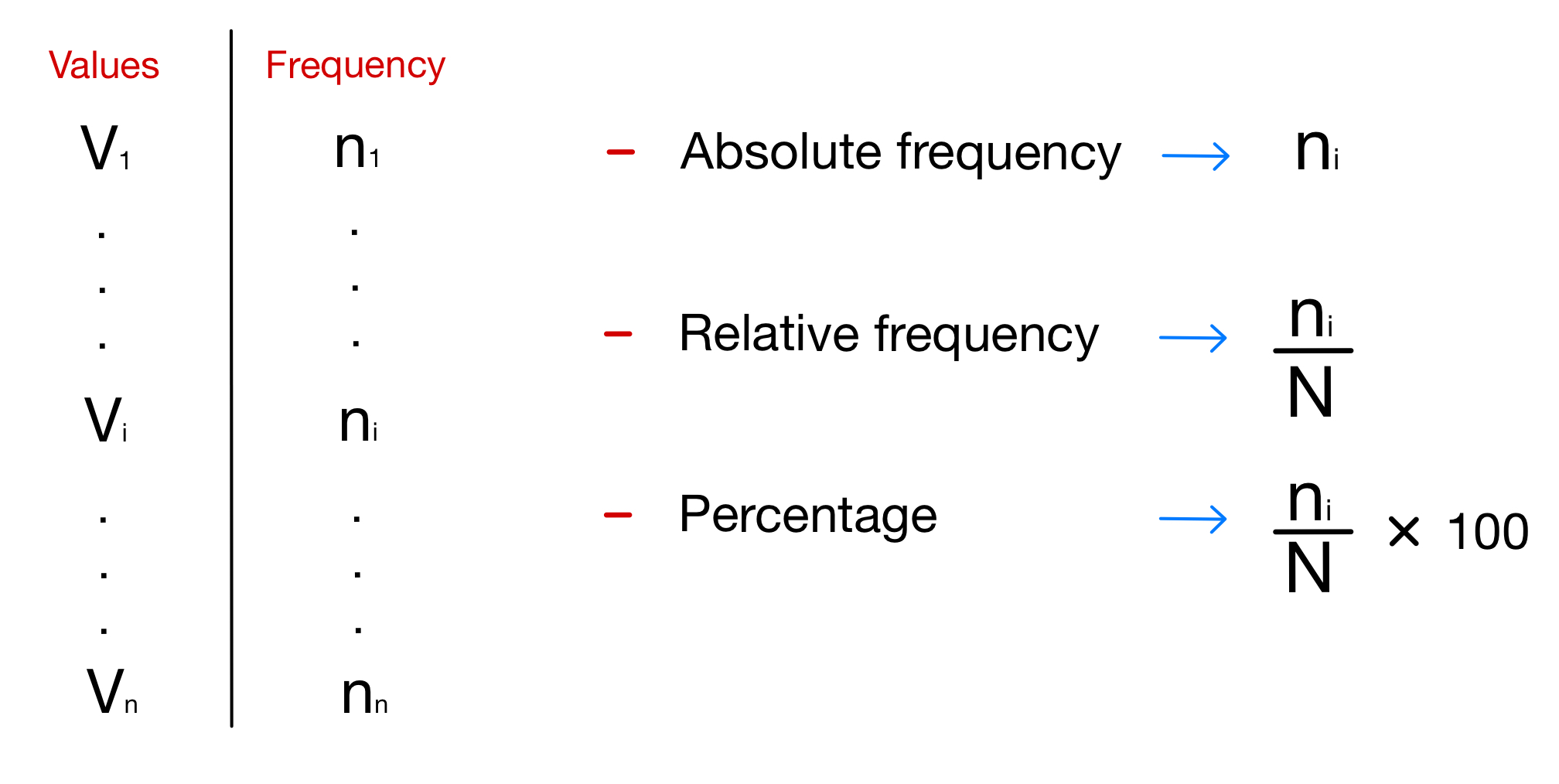
Notice how the frequency of each value can be represented in 3 ways: we can report the absolute frequency, that is exactly the number of times that value appears, we can report the relative frequency, obtained dividing the absolute frequency for the cardinality of the statistical population we consider, or we can report the percentage, obtained multiplying the relative frequency by 100.

A multivariate distribution, instead, refers to more than one attribute: for each possible combination of values we can have for the attributes we chose, the distribution shows the frequency of the units in the population that have simultaneously the considered values for the chosen attributes. To represent a multivariate distributions we use $n$-dimensional tables called contingency tables, where $n$ is the number of attributes I am considering. Of course, it’s difficult to graphically represent a contingency table if $n > 3$. In the following image, we represent a bivariate distribution, that is a multivariate distribution that refers to two attributes:

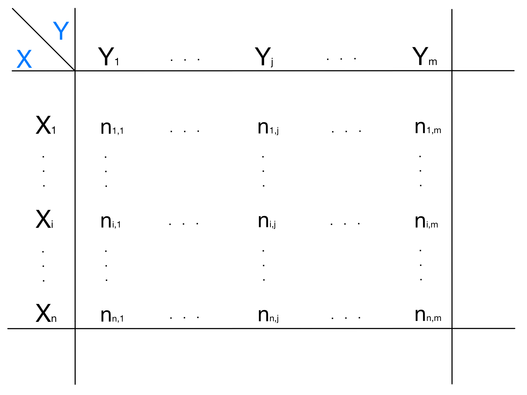
We can notice how this distribution is very different from the univariate: the table consists in a matrix of $n$ rows and $m$ columns. For each row I have a possible value for the attribute $X$, while for each column I have a possible value for the attribute $Y$. In the cell $(i,j)$ of the matrix we have the frequency of the statistical units that simultaneously have $X_{i}$ as the value for attribute $X$ and $Y_{j}$ as the value for attribute $Y$.

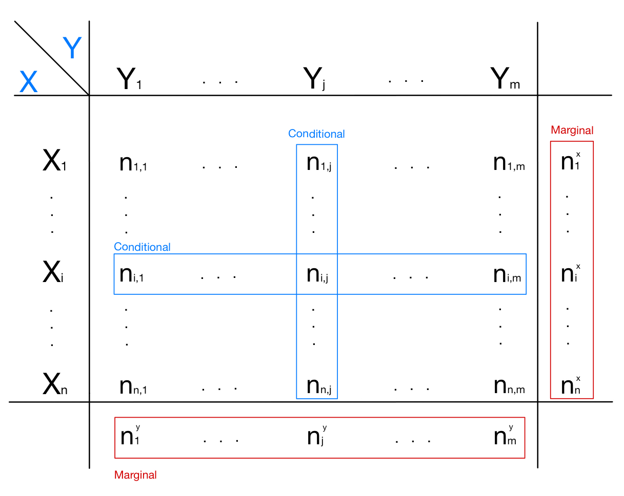
The bivariate distribution gives us the possibility to define two important new concepts: the marginal distribution and the conditional distribution. Given a bivariate contingency table, we can sum all the values on each row and obtain an additional column:

\[\sum_{j=1}^m n_{i,j} = n_i^x\]

In the same way, we can sum all the values on each column and obtain an additional row:

\[\sum_{i=1}^n n_{i,j} = n_j^y\]

This additional column and this additional row are called marginal distributions respectively of $X$ and $Y$, and are so called because they are at the margin of the table. It’s easy to see that the marginal distribution of $X$ is the univariate distribution of $X$, as the marginal distribution of $Y$ is the univariate distribution of $Y$. We can then see that a bivariate table contains much more informations than a univariate table, because it contains the univariate providing also more informations.

We can now, instead, consider a single row or a single column from the table. A single column (or row) is also called conditional distribution of $X$ (or $Y$): this because it represents the univariate distribution of $X$ (or $Y$), conditioned on a specific value of attribute $Y$ (or $X$). This can be better explained with an example: if we take the column $j$ from the table, what we will obtain is the frequency distribution of all the possible values assumed by $X$, as long as the statistical units that we consider have the value $Y_j$ for the attribute $Y$. Conditioned distributions are very important for statistical analysis: we can confront them with the univariate distribution of the same attribute, understanding if a relationships between a certain value of an attribute and the distribution of another one exists.

In the image below are represented examples of marginal and conditional distributions:

References
[1] https://www.mygreatlearning.com/blog/understanding-distributions-in-statistics/
[2] https://www.kaggle.com/code/nowke9/statistics-2-distributions
[3] https://en.wikipedia.org/wiki/Frequency_(statistics)